Tutorial: Getting Started¶

(Sigvald Marholm)

In this tutorial, we will carry out a 2D simulation of the current collected by a cylindrical Langmuir probe in non-drifting, non-magnetized, Maxwellian proton-electron plasma. The physical parameters of the problem is given below:

Parameter	Value
Ion/electron density	$10^{11}\,\mathrm{m^{-3}}$
Ion/electron temperature	$3000\,\mathrm{K}$
Electron Debye length	approx. $12\,\mathrm{mm}$
Probe radius	$1\,\mathrm{mm}$
Probe voltage	$3\,\mathrm{V}$

We start by making a new directory for the project, and make a symbolic link to the interaction executable in this folder (modify paths as necessary):

cd ~
mkdir -p Projects/tutorials/basic
cd Projects/tutorials/basic
ln -s ~/punc++/interaction/build/interaction

If using a system-wide installation of PUNC++, you can omit creating a symbolic link.

1. Mesh generation¶

Let’s start by creating a mesh. For a 2D simulation of a cylindrical probe the probe is represented by a circular, interior boundary. We shall also use a circlular exterior boundary. It is an assumption of the underlying numerical methods that the exterior boundary is in the background plasma and is not affected by any local perturbations in the electric potential. This makes it necessary for the outer boundary to be outside the sheath of the probe. The closer the outer boundary is to the probe, the less valid the assumption becomes, and the more it limits the accuracy of the simulation. On the other hand, increasing the domain size increases the cost of the simulation. The mesh gets bigger, and more simulation particles are needed to maintain the same density of particles in the domain. It may in fact also be necessary to run the simulation for a longer physical time in order to reach a sufficiently steady state. This is because the domain is uniformly filled with particles before the simulation starts, and rather violent, unphysical transients occur where the plasma is perturbed, e.g. where the sheath should be. These transients may cause waves which takes a long time to settle. In improving the accuracy of a simulation, one should attempt to improve the limiting factor, which may or may not be the radius of the outer boundary. Finding the right set of simulation parameters requires some experimentation. We will use an outer boundary of 100mm radius.

This geometry can be created either using the Gmsh Graphical User Interface (GUI), or it can be specified directly in a text file for Gmsh to read. We shall call our geometry file cylinder.geo:

ri = 0.001;   // Inner radius
ro = 0.1;     // Outer radius
resi = ri/5;  // Inner resolution
reso = 0.006; // Outer resolution

Point(1) = {  0,   0, 0, resi};
Point(2) = {+ro,   0, 0, reso};
Point(3) = {-ro,   0, 0, reso};
Point(4) = {  0, +ro, 0, reso};
Point(5) = {  0, -ro, 0, reso};
Point(6) = {+ri,   0, 0, resi};
Point(7) = {-ri,   0, 0, resi};
Point(8) = {  0, +ri, 0, resi};
Point(9) = {  0, -ri, 0, resi};

Circle(1) = {2, 1, 4};
Circle(2) = {4, 1, 3};
Circle(3) = {3, 1, 5};
Circle(4) = {5, 1, 2};
Circle(5) = {6, 1, 8};
Circle(6) = {8, 1, 7};
Circle(7) = {7, 1, 9};
Circle(8) = {9, 1, 6};

Physical Line(1) = {2, 1, 4, 3}; // Exterior
Physical Line(2) = {5, 6, 7, 8}; // Interior

// Optional
Line Loop(1) = {2, 3, 4, 1};
Line Loop(2) = {5, 6, 7, 8};
Plane Surface(1) = {1, 2};
Physical Surface(3) = {1};

On the first four lines variables are defined for the inner and outer radii, as well as the resolution of the mesh on the inner and outer boundaries. The resolution will vary continually between the boundaries. The resolution must be sufficiently fine to resolve any characteristic lengths of the physics involved. The outer boundary must therefore have a resolution not much bigger than the electron Debye length, whereas the inner boundary must in addition be sufficiently fine to resolve the circular cross-section of the probe. Insufficiently resolving the electron Debye length is known to cause numerical heating of the plasma on rectangular meshes, and it is reasonable to expect simlar effects for unstructured meshes. Since we are mostly interested in what happens close to the probe, we can often get away with a resolution that is actually somewhat bigger than the Debye length at the outer boundary.

The lines starting with Point defines a point in the center of the domain, as well as to the north, east, south and west of the center, on both boundaries. Each boundary is made up of four circle arcs (Circle) connected between these points.

It is important that the proper Physical Groups are created in Gmsh. PUNC++ needs one physical group for each boundary (Physical Lines in 2D or Physical Surfaces in 3D). Note that it is mandatory that the exterior boundary has the lowest id number of all boundaries since this is how PUNC++ knows which boundary is the exterior one. It is also possible to define a physical group for the domain (Physical Surface in 2D or Physical Volume in 3D), but this is optional.

Hint: For larger geometries it can be difficult to keep track of all line in a text editor. The author prefers to define the variables and the points in text, and subsequently opening it in Gmsh to connect arcs and lines between the points.

To generate the mesh from the GUI, run Mesh -> 2D. The mesh can be saved using File -> Save Mesh, and it will automatically be named cylinder.msh. If, however, you use Gmsh 4, the default .msh format is of a newer variety than is incompatible with the dolfin-convert tool we shall use later. In this case, you must go to File -> Export, and export it as cylinder.msh. You will be asked to choose format, and should choose Version 2 - ASCII.

The mesh can also be generated and saved directly from the terminal:

$ gmsh -2 -format msh2 cylinder.geo

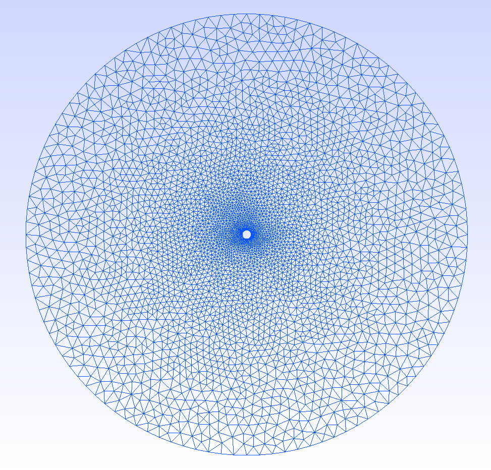
-format msh2 makes sure it is saved in the correct format, and -2 means that it is a 2D mesh. For a 3D mesh it would be -3 instead. The mesh is named cylinder.msh and should look something like this when opened in Gmsh:

The finite element approximation of the fields will be better the less sliver the cells in the mesh are. A gamma factor of 1 indicates a completely equilateral/regular cell, whereas a gamma of 0 indicates a degenerate cell. The quality of the mesh can be inspected from Gmsh by clicking Tools -> Statistics and then Update. The average, minimum and maximum gamma factor should now be displayed, and it is possible to plot the distribution of the gamma values. It may look something like this:

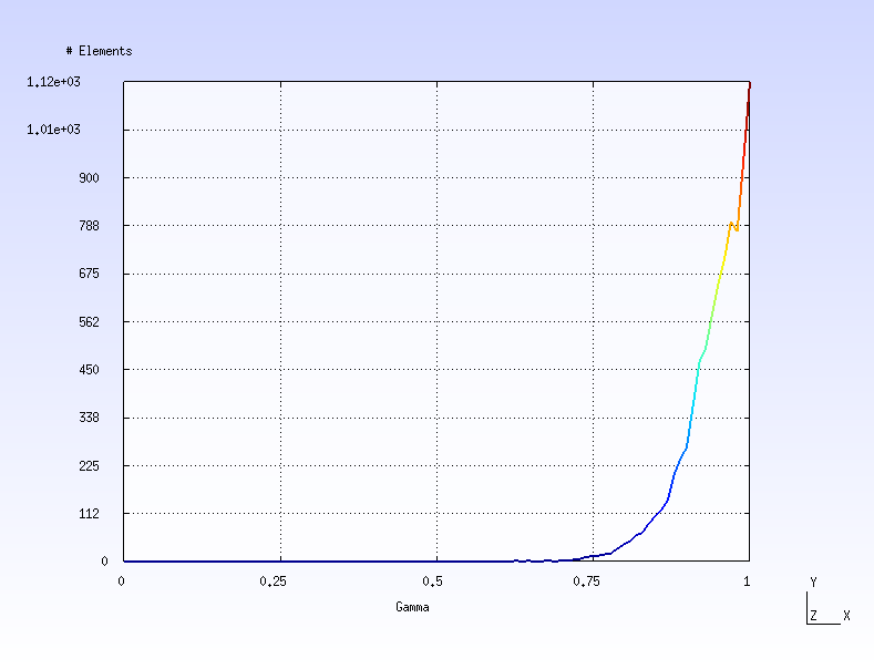
Make sure most cells are above 0.3 and that the minimum value is not zero, i.e., that there are no degenerate cells.

Mesh files must be in either DOLFIN XML or HDF5 formats. To convert the Gmsh mesh, use FEniCS’s own conversion tool:

$ dolfin-convert cylinder.msh cylinder.xml

You should now have the files cylinder.xml, cylinder_facet_region.xml and possibly also cylinder_physical_region.xml. The first file is the mesh itself, whereas the latter two contain the physical groups for the boundaries and the domain, respectively.

2. Running the simulation¶

The interaction executable loads simulation settings from an ini file which we shall call setup.ini and put in the same folder as the mesh:

mesh = cylinder.xml

[time]
stop = 1e-6 s

[species] # electron
charge = -1 e
mass = 1 me
density = 1e11
temperature = 3000 K
amount = 5e5

[species] # proton
charge = 1 e
mass = 1 amu
density = 1e11
temperature = 3000 K
amount = 5e5

[objects]
vsource = -1 0 3

[diagnostics]
period_phi = 3e-9 s

Most settings in this file are pretty self-explanatory. The mesh is found in cylinder.xml and the mesh is run for $1\,\mathrm{\mu s}$ . Note that cylinder_facet_region.xml is also used although not explicitly mentioned. The simulation consists of electrons and protons. In particular, it contains $5\cdot 10^5$ macroparticles of each. Notice also that some settings take suffixes (units). Mass can for instance be specified in both electron masses (me) or atomic mass units (amu).

The exterior boundary should, as mentioned, have the lowest id in the .geo file. The second lowest boundary id is taken to be object 0, the third lowest id object 1, and so forth. The objects are always perfect electric conductors, and by default their floating potential will be self-consistently determined from collected charges. In our case, however, we would like to fix the potential of the cylinder to 3V. We do this by adding a voltage source (vsource) between system ground (-1) and the object (0) of 3V. Multiple voltage and current sources can be defined between two objects, or between objects and sytem ground by adding several vsource and isource entries under the [objects] section.

For this simulation we have also included an optional diagnostics, namely that the electric potential be saved every 3 nanoseconds.

Finally, to run the simulation, type:

$ ./interaction setup.ini

Omit ./ if using system-wide installation. After the simulation is complete, three dat files should appear. history.dat contains time-series diagnostics. population.dat contains all the particles at the end of the simulation and state.dat contains auxiliary variables necessary to continue the simulation from where it stopped. After having a look at the data, we would probably conclude that $1\,\mathrm{\mu s}$ was a bit short, and decide to increase it to $2\,\mathrm{\mu s}$ . We chould then simply change setup.ini and execute the program again to pick up the simulation where we left off. It is also possible to stop a simulation gracefully by pressing Ctrl+C once, and continuing the simulation later. Pressing Ctrl+C a second time kills the program instantly, without possibility for continuation. To restart a simulation from scratch, remove one of the dat files.

It is also possible to override a setting in an ini file by command line arguments. For instance, to expand the simulation time, we could also execute:

$ ./interaction setup.ini --time.stop "2e-6 s"

interaction supports a wide range of settings, each of which can be set either in the ini file or as a command line argument. The full list is available from:

$ ./interaction --help

3. Inspecting the results¶

Time-series are stored in a tabulated ASCII file history.dat. The first few lines for our simulation is demonstrated below:

#:xaxis	t
#:name	n	t	ne	ni	KE	PE	V[0]	I[0]	Q[0]
#:long	timestep	time	"number of electrons"	"number of ions"	"kinetic energy"	"potential energy"	voltage	current	charge
#:units	1	s	m**(-3)	m**(-3)	J	J	V	A/m	C
0	0.0000000000000000e+00	5.0000000000000000e+05	5.0000000000000000e+05	2.5933134548417018e-10	0.0000000000000000e+00	2.9999999999999858e+00	0.0000000000000000e+00	3.1347679114736289e-11
1	9.4835501346177436e-10	5.0006300000000000e+05	4.9998800000000000e+05	2.5935999910087600e-10	0.0000000000000000e+00	2.9999999999999876e+00	-9.4912670089575748e-06	3.1344180209498419e-11
2	1.8967100269235487e-09	5.0002900000000000e+05	4.9998700000000000e+05	2.5939544396473562e-10	0.0000000000000000e+00	2.9999999999999862e+00	-2.2146289687567667e-05	3.1344267993384300e-11

The first six columns shows the time-step, the physical time at the time-step, the number of negatively charged particles (electrons), the number of positively charged particles (ions), total kinetic energy of the particles, and total potential energy of the particles, respectively. Subsequently follows three columns for each objects, its voltage, collected current, and charge.

The commented lines in the header follows the syntax of Metaplot, which allows for easy visualization. To plot the current collected by the probe (which is object zero):

$ mpl history.dat "I[0]"

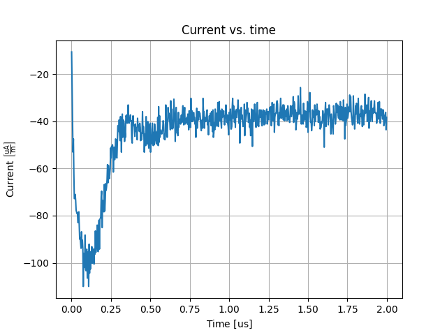
The current collected should according to OML theory be $-35.3\,\mathrm{\mu A}$ . Since the simulation is quite rough it is a bit hard to see how close it actually is. Let us perform an Exponential Moving Average (EMA) with a relaxation time of $0.1\,\mathrm{\mu s}$ and compare to the OML theory:

$ mpl history.dat "truth(-34.3e-6)(ema(1e-7)(I[0]))"

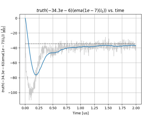
This is not too bad given that the simulation is quite rough. Let us also plot the number of electrons and ions:

$ mpl history.dat ne ni

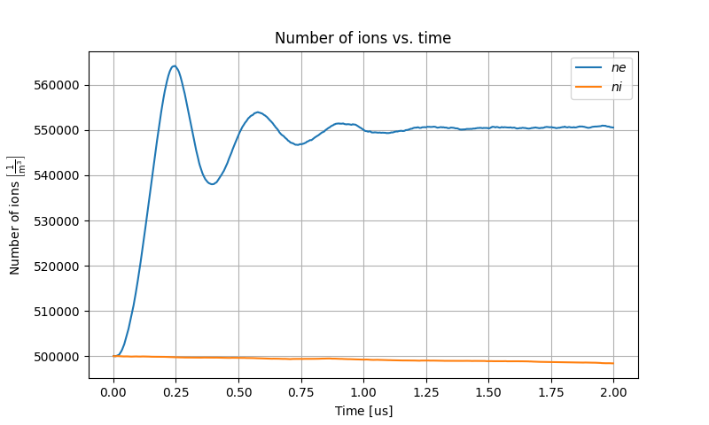
The number of electrons seems to have reached steady-state. The number of ions have not had time to change very much. We not that Metaplot is a very experimental program at this stage. We do not delve further into it.

Finally, let us have a look at the electric potential we stored every $3\,\mathrm{ns}$ . The field quantities are stored in the fields folder in VTK format, and is easily visualized using ParaView. To open the electric potential:

$ paraview fields/phi.pvd

Inside ParaView, click Apply and then the green play symbol to start an animation. It should look something like the following:

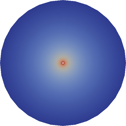
Initially the plasma is uniformly distributed and the potential is that of a cylinder in vacuum. As the sheath starts forming due to the surrounding plasma, acoustic shock waves emerges and travel outwards, eventually forming standing waves between the boundaries before they die out and the correct solution is arrived at at steady-state.